Categorical variable encoding using aggregated mean and std
Introduction
Preprocessing cartegorical features is no easy task. The most basic technique would probably be one-hot-encoding method. However, one-hot-encoding is not efficient whenever the number of features is large.
In this article, We will learn how to handle many categorical features effectively even though the number of features is large. This technique was used by the winner of Kaggle’s “IEEE-CIS Fraud Detection” competition and can be found at here.
How the Magic Works (source)
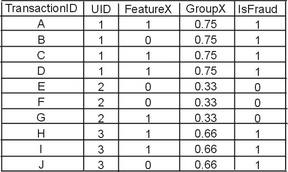
The magic is two things. First we need a UID variable to identify clients (credit cards). Second, we need to create aggregated group features. Then we remove UID. Suppose we had 10 transactions A, B, C, D, E, F, G, H, I, J as below.

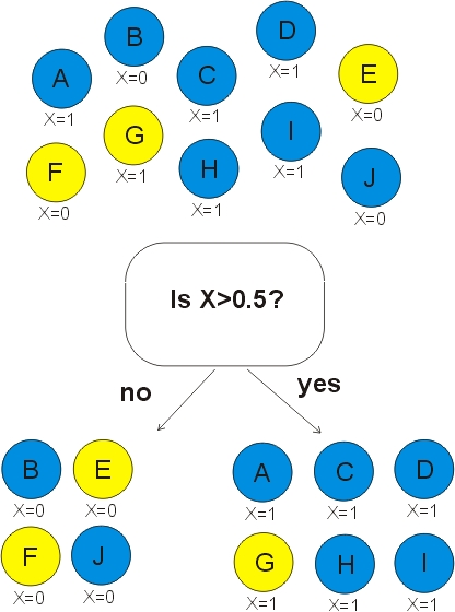
If we only use FeatureX, we can classify 70% of the transactions correctly. Below, yellow circles are isFraud=1 and blue circles are isFraud=0 transactions. After the tree model below splits data into left child and right child, we predict isFraud=1 for left child and isFraud=0 for right child. Thus 7 out of 10 predictions are correct.

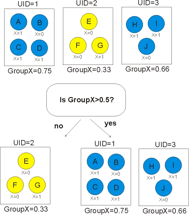
Now suppose that we have a UID which defines groups and we make an aggregated feature by taking the average of FeatureX within each group. We can now classify 100% of the transactions correctly. Note that we never use the feature UID in our decision tree.

Data Explanation
In the original dataframe, there are 392 features including both numeric features and categrical features.

Feature Information
Transaction Table
- TransactionDT: timedelta from a given reference datetime (not an actual timestamp)
- TransactionAMT: transaction payment amount in USD
- ProductCD: product code, the product for each transaction
- card1 - card6: payment card information, such as card type, card category, issue bank, country, etc.
- addr: address
- dist: distance
- P_ and (R__) emaildomain: purchaser and recipient email domain
- C1-C14: counting, such as how many addresses are found to be associated with the payment card, etc. The actual meaning is masked.
- D1-D15: timedelta, such as days between previous transaction, etc.
- M1-M9: match, such as names on card and address, etc.
- Vxxx: Vesta engineered rich features, including ranking, counting, and other entity relations.
Categorical Features:
- ProductCD
- card1 - card6
- addr1, addr2
- Pemaildomain Remaildomain
- M1 - M9
Identity Table
Variables in this table are identity information – network connection information (IP, ISP, Proxy, etc) and digital signature (UA/browser/os/version, etc) associated with transactions. They’re collected by Vesta’s fraud protection system and digital security partners. (The field names are masked and pairwise dictionary will not be provided for privacy protection and contract agreement)
Categorical Features:
- DeviceType
- DeviceInfo
- id12 - id38
Read data
import numpy as np, pandas as pd, os, gc
from sklearn.model_selection import GroupKFold
from sklearn.metrics import roc_auc_score
import matplotlib.pyplot as plt
import seaborn as sns

# LOAD TRAIN
X_train = pd.read_csv('../input/ieee-fraud-detection/train_transaction.csv',index_col='TransactionID', nrows=10000)
train_id = pd.read_csv('../input/ieee-fraud-detection/train_identity.csv',index_col='TransactionID', nrows=10000)
X_train = X_train.merge(train_id, how='left', left_index=True, right_index=True)
# LOAD TEST
X_test = pd.read_csv('../input/ieee-fraud-detection/test_transaction.csv',index_col='TransactionID', nrows=10000)
test_id = pd.read_csv('../input/ieee-fraud-detection/test_identity.csv',index_col='TransactionID', nrows=10000)
X_test = X_test.merge(test_id, how='left', left_index=True, right_index=True)
# TARGET
y_train = X_train['isFraud'].copy()
del train_id, test_id, X_train['isFraud'];
x = gc.collect()
# PRINT STATUS
>>>print('Train shape',X_train.shape,'test shape',X_test.shape)
Train shape (10000, 432) test shape (10000, 432)
Basic Feature Engineering
We use pandas’s factorize function to convert categorical variables into numeric variables.
Pandas.factorize
pandas.factorize(values, sort=False, order=None, na_sentinel=-1, size_hint=None)
Encode the object as an enumerated type or categorical variable.
>>> labels, uniques = pd.factorize(['b', 'b', 'a', 'c', 'b'])
>>> labels
array([0, 0, 1, 2, 0])
>>> uniques
array(['b', 'a', 'c'], dtype=object)
The next things to do are:
- (factorize) Convert categorical variables using pandas’ factorize function.
- (memory reduce) If the max value is 32000 or higher, the data type is converted to ‘int32’ type, otherwise it is converted to ‘int32’.
- (positive) Change all numeric values to zero or above.
- (NAN to -1) Convert all NAN values to -1.
# LABEL ENCODE AND MEMORY REDUCE
for i,f in enumerate(X_train.columns):
    # FACTORIZE CATEGORICAL VARIABLES
    if (np.str(X_train[f].dtype)=='category')|(X_train[f].dtype=='object'):
        df_comb = pd.concat([X_train[f],X_test[f]],axis=0)
        df_comb,_ = df_comb.factorize(sort=True)        # (factorize)
        if df_comb.max()>32000: print(f,'needs int32')  # (memory reduce)
        X_train[f] = df_comb[:len(X_train)].astype('int16')
        X_test[f] = df_comb[len(X_train):].astype('int16')

    # SHIFT ALL NUMERICS POSITIVE. SET NAN to -1
    elif f not in ['TransactionAmt','TransactionDT']:
        mn = np.min((X_train[f].min(),X_test[f].min()))
        X_train[f] -= np.float32(mn)                   # (positive)
        X_test[f] -= np.float32(mn)                    # (NAN to -1)
        X_train[f].fillna(-1,inplace=True)
        X_test[f].fillna(-1,inplace=True)
Since this is time series data, we use the first 75% as the train set and the latter 25% as the validation set.
# CHRIS - TRAIN 75% PREDICT 25%
idxT = X_train.index[:3*len(X_train)//4]
idxV = X_train.index[3*len(X_train)//4:]
We will now test the performance of the original version of the XGBoost model.
import xgboost as xgb
print("XGBoost version:", xgb.__version__)

clf = xgb.XGBClassifier(
    n_estimators=2000,
    max_depth=12,
    learning_rate=0.02,
    subsample=0.8,
    colsample_bytree=0.4,
    missing=-1,
    eval_metric='auc',
    # USE CPU
    nthread=4,
    tree_method='hist'
    # USE GPU
    #tree_method='gpu_hist'
)
h = clf.fit(X_train.loc[idxT], y_train[idxT],
    eval_set=[(X_train.loc[idxV],y_train[idxV])],
    verbose=50, early_stopping_rounds=100)

feature_imp = pd.DataFrame(sorted(zip(clf.feature_importances_,cols)), columns=['Value','Feature'])
plt.figure(figsize=(20, 10))
sns.barplot(x="Value", y="Feature", data=feature_imp.sort_values(by="Value", ascending=False).iloc[:50])
plt.title('XGB95 Most Important Features')
plt.tight_layout()
plt.show()
del clf, h; x=gc.collect()
The result is as follows:
XGBoost version: 0.90
[0]	validation_0-auc:0.677229
Will train until validation_0-auc hasn't improved in 100 rounds.
[50]	validation_0-auc:0.831485
[100]	validation_0-auc:0.841948
[150]	validation_0-auc:0.857862
[200]	validation_0-auc:0.860735
[250]	validation_0-auc:0.868282
[300]	validation_0-auc:0.867505
Stopping. Best iteration:
[245]	validation_0-auc:0.86896
Advanced Feature Engineering using the Magic Features
Let’s take a look at how to use the magic feature to improve the performance of the original XGBoost model.
This requires two other operations.
COMBINE FEATURES
Concatenate two string type features to create a new feature. Ex) Hyundai Card + Suwon = Hyundai Card_Suwon
GROUP AGGREGATION MEAN AND STD
Based on one feature, group the items belonging to the same class to find mean and std and add each new feature.
# COMBINE FEATURES
def encode_CB(col1,col2,df1=X_train,df2=X_test):
    nm = col1+'_'+col2
    df1[nm] = df1[col1].astype(str)+'_'+df1[col2].astype(str)
    df2[nm] = df2[col1].astype(str)+'_'+df2[col2].astype(str)
    encode_LE(nm,verbose=False)
    print(nm,', ',end='')

# GROUP AGGREGATION MEAN AND STD
# https://www.kaggle.com/kyakovlev/ieee-fe-with-some-eda
def encode_AG(main_columns, uids, aggregations=['mean'], train_df=X_train, test_df=X_test,
              fillna=True, usena=False):
    # AGGREGATION OF MAIN WITH UID FOR GIVEN STATISTICS
    for main_column in main_columns:
        for col in uids:
            for agg_type in aggregations:
                new_col_name = main_column+'_'+col+'_'+agg_type
                temp_df = pd.concat([train_df[[col, main_column]], test_df[[col,main_column]]])
                if usena: temp_df.loc[temp_df[main_column]==-1,main_column] = np.nan
                temp_df = temp_df.groupby([col])[main_column].agg([agg_type]).reset_index().rename(
                                                        columns={agg_type: new_col_name})

                temp_df.index = list(temp_df[col])
                temp_df = temp_df[new_col_name].to_dict()

                train_df[new_col_name] = train_df[col].map(temp_df).astype('float32')
                test_df[new_col_name]  = test_df[col].map(temp_df).astype('float32')

                if fillna:
                    train_df[new_col_name].fillna(-1,inplace=True)
                    test_df[new_col_name].fillna(-1,inplace=True)

                print("'"+new_col_name+"'",', ',end='')

# LABEL ENCODE
def encode_LE(col,train=X_train,test=X_test,verbose=True):
    df_comb = pd.concat([train[col],test[col]],axis=0)
    df_comb,_ = df_comb.factorize(sort=True)
    nm = col
    if df_comb.max()>32000:
        train[nm] = df_comb[:len(train)].astype('int32')
        test[nm] = df_comb[len(train):].astype('int32')
    else:
        train[nm] = df_comb[:len(train)].astype('int16')
        test[nm] = df_comb[len(train):].astype('int16')
    del df_comb; x=gc.collect()
    if verbose: print(nm,', ',end='')
We use the function ‘encode_CB’ to combine columns card1+addr1, card1+addr1+P_emaildomain
encode_CB('card1','addr1')
encode_CB('card1_addr1','P_emaildomain')
Use the function ‘encode_LE’ to get the aggregated mean and std for the feature created above and add it as new features.
encode_AG(['TransactionAmt','D9','D11'],['card1','card1_addr1','card1_addr1_P_emaildomain'],['mean','std'],usena=True)
Now let’s run XGBoost with the input data containing the newly added features.
XGBoost version: 0.90
[0]	validation_0-auc:0.673694
Will train until validation_0-auc hasn't improved in 100 rounds.
[50]	validation_0-auc:0.883513
[100]	validation_0-auc:0.930568
[150]	validation_0-auc:0.965679
[200]	validation_0-auc:0.978922
[250]	validation_0-auc:0.979067
[300]	validation_0-auc:0.977088
Stopping. Best iteration:
[218]	validation_0-auc:0.979635
Great! The score has increased from 0.86896 -> 0.979635.